Logistic regression is one of the most famous ML models used in supervised learning settings. Despite the term “regression” in its name, this model is mostly used for classification tasks. An important distinction between logistic regression and another very popular supervised learning model, linear regression, is that the response variable is categorical for the former but continuous for the latter.

Most ML researchers use this model as a baseline in many supervised learning tasks because of its simplicity. In fact, for most practical applications, logistic regression turns out to be the best performing model even compared to more complex deep learning models. For example, it is the best model to predict outcomes in NCAA mens basketball in a data science competition a few years back.

Definition

Standard logistic regression is used for binary classification tasks although it can be extended to multiclass settings (> 2 labels). Here’s its formal definition:

Given $m$ training examples $\{ (x^{(1)}, y^{(1)}), \thinspace (x^{(2)}, y^{(2)}), \thinspace…\thinspace, (x^{(m)}, y^{(m)}) \}$, logistic regression model outputs corresponding predicted values $\{ \hat{y}^{(1)}, \thinspace \hat{y}^{(2)}, \thinspace…\thinspace, \hat{y}^{(m)} \}$ where $0 \leq \hat{y}^{(i)} \leq 1$ can be interpreted as probability of example (i) belonging to class 1 (i.e. $y^{(i)} = 1$)

$$ \hat{y}^{(i)} = P(y^{(i)} = 1 \thinspace | \thinspace x^{(i)}) = \sigma (w^Tx^{(i)} + b)$$

where $\sigma$ is sigmoid function (see below), $w$, $b$ are model parameters such that $w \in \mathbb{R}^{n_{x}}$, $b \in \mathbb{R}$, each training example is represented by $n_x$-dimentional vector $x^{(i)}$, $y$ can either be 0 or 1 to indicate two classes that each data case can fall into

Sigmoid function

Sigmoid function, denoted by $\sigma$, is used as activation function for logistic regression. It has this following form for a real-valued input z:

$$ \sigma (z) = \frac{1}{1 + e^{-z}} $$

Here’s its graphical representation

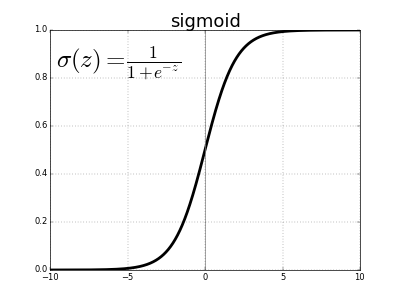
Clearly, sigmoid function outputs are bounded between 0 and 1. These outputs can be interpreted as probabilities of data cases belonging to class $y = 1$.

In other words, for a given data case (i), if its predicted $\hat{y}^{(i)} = \sigma (z^{(i)}) = \sigma (w^Tx^{(i)} + b) > 0.5$, then the model predicts that this data case belongs to class $y = 1$

How is logistic regression fit to training data?

Given a cost function (also called objective function) of $w$ and $b$, the logistic regression model’s goal is to find suitable values of $w$ and $b$ such that this cost function’s value is as small as possible.

This cost function is not unique to logistic regression. Generally, all (supervised) ML models have associated cost functions as functions of the model parameters. A cost function quantifies how well a model is performing against the given training data set, i.e. how far off our predicted response values $\hat{y}^{(i)}$’s are from our ground truth response labels $y^{(i)}$’s.

So what does this cost function look like for logistic regression?

For a single example (i), we have $$ \ell (y, \hat{y}) = - (y * log(\hat{y}) + (1-y) * log(1 - \hat{y})) $$

Side note: this cost function is also known as cross entropy loss

Thus the overal cost function over all training examples is just the average of these individual losses

$$ J(w, b) = \frac{-1}{m} \sum_{i=1}^{m}y * log(\hat{y}) + (1-y) * log(1 - \hat{y}) $$

So how does logistic regression model find values $w$, $b$ to minimize the value of this cost function?

Well, through a training algorithm called gradient descent.

Those with Calculus background will find this idea familiar: the minimum of the objective function is (hopefully) found by iteratively lowering its value through updating its model parameters in the direction of the cost function’s gradient (or partial derivatives) w.r.t. these parameters.

Details about how to mathematically derive this gradient is left in this post

This iterative process is bounded by the number of iterations specified by the model builder or when the difference between cost function values in consecutive steps satisfies some threshold.

This process can also be fine-tuned by a hyperparameter called the learning rate (usually denoted by $\alpha$), which controls how fast this process should proceed. There’s a couple caveat about how to set this hyperparameter: too big and there might be a chance your logreg model is going to overshoot its minimum and never converge. Or too small and your model takes forever to learn.

There’s no hard and fast rule regarding how to set this hyperparameter appropriately. I will cover this topic in depth in a future post on model validation techniques.

The logistic regression model parameter update can be summarized as follows

Repeat {
    w := w - learning_rate * (gradient w.r.t w)
    b := b - learning_rate * (gradient w.r.t b)
}

After this process ends, our final values for parameters $w$ and $b$ will be used to predict which class any unforeseen data case will fall into.